New views can be created by splitting the
view frame using the SplitView controls at the top-right corner of the
view frame. Splitting a view divides the view into two equal parts, either
vertically or horizontally, based on the button used for the split.
On splitting a view, an empty frame with buttons for all known types
of views is shown. Simply click on one of those buttons to create a new view of
a chosen type.
You can make the views of the active layout fullscreen by using View > Fullscreen (layout) (or using the F11 key).
You can also make the active view alone fullscreen by using View > Fullscreen (active view) (or using CTRL + F11 keys).
To return back to the normal mode, use the Esc key.
# Create a view>>>view1=CreateRenderView()# Create a second view>>>view2=CreateRenderView()# Check if view2 is the active view>>>view2==GetActiveView()True# Make view1 active>>>SetActiveView(view1)>>>view1==GetActiveView()True
# To get exisiting tabs/layouts>>>layouts=GetLayouts()>>>print(layouts){('ViewLayout1','264'):<paraview.servermanager.ViewLayoutobjectat0x2e5b7d0>}# To get layout corresponding to a particular view>>>print(GetLayout(view))<paraview.servermanager.ViewLayoutobjectat0x2e5b7d0># If view is not specified, active view is used>>>print(GetLayout())<paraview.servermanager.ViewLayoutobjectat0x2e5b7d0># To create a new tab>>>new_layout=servermanager.misc.ViewLayout(registrationGroup="layouts")# To split the cell containing the view, either horizontally or vertically>>>view=GetActiveView()>>>layout=GetLayout(view)>>>locationId=layout.SplitViewVertical(view=view,fraction=0.5)# fraction is optional, if not specified the frame is split evenly.# To assign a view to a particular cell.>>>view2=CreateRenderView()>>>layout.AssignView(locationId,view2)
Since the visualization process in general focuses on reducing data to
generate visual representations, the rendering (broadly speaking) is less time-intensive
than the actual data processing. Thus, changing properties that affect
rendering are not as compute-intensive as transforming the data itself. For example,
changing the color on a surface mesh is not as expensive as generating the mesh
in the first place. Hence, the need to Apply such properties becomes less
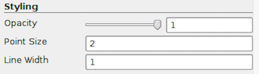
relevant. At the same time, when changing display properties such as opacity,
you may want to see the result as you change the property to decide on the final
value. Hence, it is desirable to see the updates immediately.
# 1. Save reference when a view is created>>>view=CreateView("RenderView")# 2. Get reference to the active view.>>>view=GetActiveView()
ビューで使用できるプロパティは、ビューのタイプによって異なります。 help 関数を使用すると、使用可能なプロパティを見つけることができます。
>>> view=CreateRenderView()>>> help(view) Help on RenderView in module paraview.servermanager object:class RenderView(Proxy) | View proxy for a 3D interactive render | view. | | ---------------------------------------------------------------------- | Data descriptors defined here: | | CenterAxesVisibility | Toggle the visibility of the axes showing the center of | rotation in the scene. | | CenterOfRotation | Center of rotation for the interactor. | ...# Once you have a reference to the view, you can then get/set the properties.# Get the current value>>> print(view.CenterAxesVisibility)1# Change the value>>> view.CenterAxesVisibility=0
# Using SetDisplayProperties/GetDisplayProperties to access the display# properties for the active source in the active view.>>>print(GetDisplayProperties("Opacity"))1.0>>>SetDisplayProperties(Opacity=0.5)
# Get display properties object for the active source in the active view.>>>disp=GetDisplayProperties()# You can also save the object returned by Show.>>>disp=Show()# Now, you can directly access the properties.>>>print(disp.Opacity)0.5>>>disp.Opacity=0.75
help メソッドを使用して、表示オブジェクトで使用可能なプロパティを検出できます。
>>> disp=Show()>>> help(disp)>>> help(a)Help on GeometryRepresentation in module paraview.servermanager object:class GeometryRepresentation(SourceProxy) | ParaView`s default representation for showing any type of | dataset in the render view. | | Method resolution order: | GeometryRepresentation | SourceProxy | Proxy | __builtin__.object | | ---------------------------------------------------------------------- | Data descriptors defined here: | | ... | | CenterStickyAxes | Keep the sticky axes centered in the view window. | | ColorArrayName | Set the array name to color by. Set it to empty string | to use solid color. | | ColorAttributeType | ...
The RenderView is the most commonly used view in ParaView. It is used to render
geometries and volumes in a 3D scene. This is the view that you typically think
of when referring to 3D visualization. The view relies on techniques to map data
to graphics primitives such as triangles, polygons, and voxels, and it renders
them in a scene.
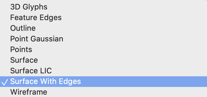
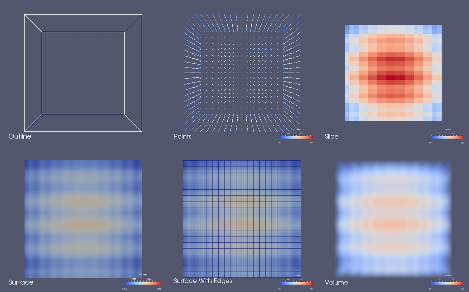
Most of the scientific datasets discussed in 3.1 章
are composed of meshes. These meshes can be mapped to graphics primitives using
several of the established visualization techniques. That is, you can compute the
outer surface of these meshes and then render that surface as filled polygons, you can
just render the edges, or you can render the data as a nebulous blob to get a better
understanding of the internal structure in the dataset. Plugins, like
DigitalRockPhysics, can provide additional ways of rendering data using advanced
techniques that provide more insight into the data.
Unless you changed the default setting, a new RenderView will be created
when paraview starts up or connects to a new server. To create a
RenderView in paraview, split or close a view, and select the
RenderView button. You can also convert a view to a RenderView (or any other
type) by right-clicking on the view's title bar and picking from the ConvertTo sub-menu. It simply closes the chosen view and creates a selected view type
in its place.
通常、ParaView では、3Dシーンを操作することになります。しかし、スライス平面や2D画像のような2Dデータセットを操作する場合もあります。そのような場合、paraview は2Dインタラクションに適したインタラクションオプションのセットを別に提供します。ビューツールバーの 2D または 3D ボタンをクリックすると、デフォルトの3Dインタラクションオプションと2Dインタラクションオプションを切り替えることができます。2Dインタラクションのデフォルトのインタラクションオプションは、以下の通りです。
Modifier
Left Button
Middle Button
Right Button
Pan
Roll
Zoom
⇧
Zoom
Zoom
Zoom To Mouse
CTRL or ⌘
Roll
Pan
Rotate
デフォルトでは、ParaView はデータを読み込む際に2Dか3Dかを判断し、それに応じてインタラクションモードを設定します。この動作は Settings ダイアログの RenderView タブにある DefaultInteractionMode 設定を変更することで行うことができます。デフォルトは "Automatic, based on the first time step" ですが、強制的にインタラクションモードを変更したい場合は、"Always 2D" または "Always 3D" に設定を変更することが可能です。
You can also change the Background used for this view. You can either set it as a
Single color or as a Gradient changing between two colors, or you can select an
Image (or texture) to use as the background.
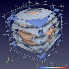
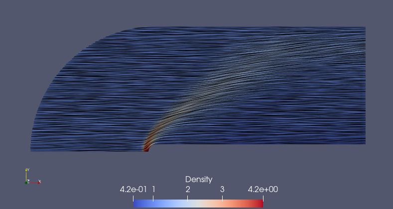
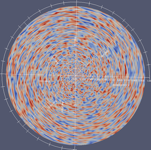
Lastly, the SurfaceLIC representation is available for surface datasets with
vector point data arrays. LIC stands for line integral convolution, which is a visualization
technique that shows the direction of flow as a noise pattern smeared in the
direction of flow.
図 4.6 An example of the SurfaceLIC representation showing the direction of a
vector data array and colored by a different scalar array showing (Density).
If instead you want to pseudocolor using an attribute array
available on the dataset, select that array name from the combo-box. For
multi-component arrays, you can pick a particular component or Magnitude to
use for scalar coloring. ParaView will automatically set up a color transfer
function it will use to map the data array to colors. The default range for the
transfer function is set up based on the TransferFunctionResetMode general
setting in the Settings dialog when the transfer function is first created.
If another dataset is later colored by a data array with the same name, the range
of the transfer function will be updated according to the AutomaticRescaleRangeMode
property in the ColorMapEditor . To reset the transfer function range to the
range of the data array in the selected dataset, you can use the Rescale
button. Remember that, despite the fact that you can set the scalar array with
which to color when rendering as Outline , the outline itself continues to use
the specified solid color.
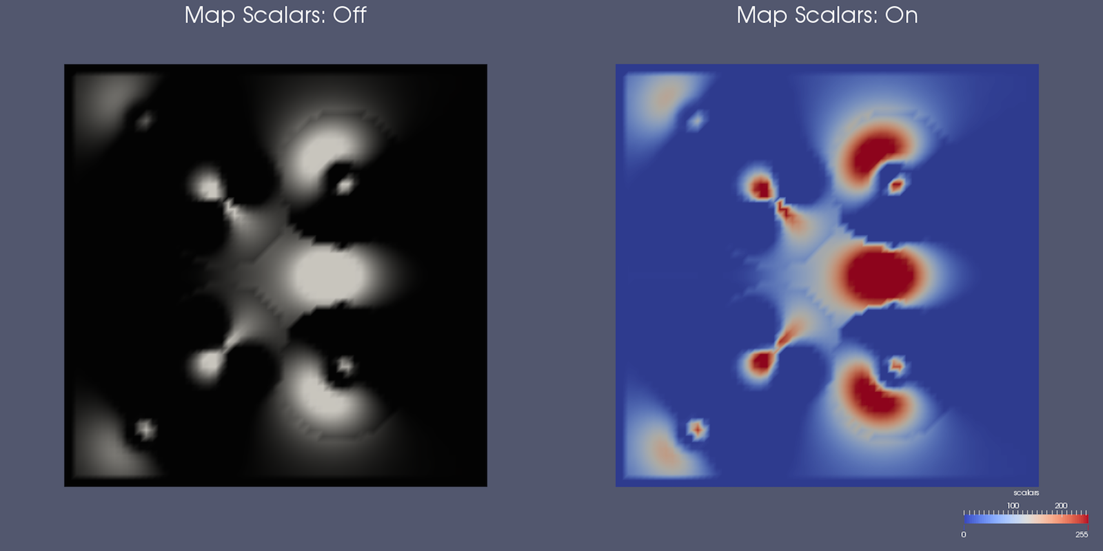
ScalarColoring properties are only relevant when you have selected a data
array with which to pseudocolor. The MapScalars checkbox affects whether a color
transfer function should be used (図 4.7).
If unchecked, and the data array can directly
be interpreted as colors, then those colors are used directly. If not, the color
transfer function will be used. A data array can be interpreted as colors if, and
only if, it is an unsigned char, float, or double array with two, three, or four
components. If the data array is unsigned char, the color values are defined between
0 and 255 while if the data array is float or double, the color values are expected
to be between 0 and 1. InterpolateScalarsBeforeMapping controls how color
interpolation happens across rendered polygons. If
on, scalars will be interpolated within polygons, and color mapping will occur
on a per-pixel basis. If off, color mapping occurs at polygon points, and colors
are interpolated, which is generally less accurate. Refer to the Kitware blog
[PatMarion] for a detailed explanation of this option.
UseNanColorForMissingArrays is a property that, if enabled, will use the special
color designated for NaN values in a dataset to also be used as the color for parts of
a composite dataset that are missing the scalars array used for color mapping.
The CoordinateShiftScaleMethod is used to choose how to normalize point coordinates
to improve rendering quality. Mesh points are sent to the GPU as single-precision float data
which can result in resolution issues due to limited precision. VTK includes a variety of
methods to normalize the point coordinates to a better range for single-precision floats
prior to sending them to the GPU. AutoShiftScale is a good setting that should work
for most datasets - it recomputes a shift and scale factor according to a heuristic involving
dataset size and position relative to the origin. AlwaysAutoShiftScale recomputes the
shift and scale every time. AutoShiftOnly only shifts the data - this is useful when
data is far away from the origin. NearFocalPlaneShiftScale and FocalPointShiftScale
works based on the current camera near clipping point and viewpoint, respectively. This makes
it the most robust setting, especially for very large datasets, but it will renormalize the
points occasionally as the camera's settings change. Renormalizing points requires reuploading
the data to the GPU, so there may be a performance cost with these last methods.
The property UseShaderReplacements enables you to customize the shader code
VTK uses for rendering by specifying shader replacements with a JSON string.
The JSON string can be a single node or an array of nodes with the following properties:
"type": specifies the type of shader the replacement is about.
It can be either "vertex", "fragment" or "geometry".
"original": specifies the original string to be replaced in the shader code.
This string is generally a pattern defined by the mapper
vtkOpenGLPolyDataMapper at specific locations of the shader
GLSL source code.
"replacement": specifies the replacement string in GLSL source code.
Note that the Json parser supports multiple lines entries.
Here's an example of a simple shader replacement (draw all the fragments in full red
color without any shading consideration):
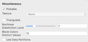
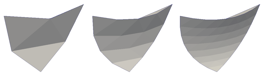
The NonlinearSubdivisionLevel property is used when rendering datasets with higher-
order elements. Use this to set the subdivision level for triangulating higher
order elements. The higher the value, the smoother the edges. This comes at the
cost of more triangles and, hence, potentially, increased rendering time.
The BlockColorsDistinctValues property sets the number
of unique colors to use when coloring multiblock datasets by block ID. Finally,
UseDataPartitions controls whether data is redistributed when it is
rendered translucently. When off (default value), data is repartitioned by the
compositing algorithm prior to rendering. This is typically an expensive
operation that slows down rendering. When this option is on, the existing data
partitions are used, and the cost of data restribution is avoided. However, if
the partitions are not sortable in back-to-front order, rendering artifacts may
occur.
>>> fromparaview.simpleimport*>>> view=CreateRenderView()# Alternatively, use CreateView.>>> view=CreateView("RenderView")
noindent Show および Hide を使用して、パイプラインモジュールによって生成されたデータをビューで表示または非表示にできます。
>>> source=Sphere()>>> view=CreateRenderView()# Show active source in active view.>>> Show()# Or specify source and view explicitly.>>> Show(source,view)# Hide source in active view.>>> Hide(source)
# Get camera from the active view, if possible.>>>camera=GetActiveCamera()# or, get the camera from a specific render view.>>>camera=view.GetActiveCamera()# Now, you can use methods on camera to move it around the scene.# Divide the camera's distance from the focal point by the given dolly value.# Use a value greater than one to dolly-in toward the focal point, and use a# value less than one to dolly-out away from the focal point.>>>camera.Dolly(10)# Set the roll angle of the camera about the direction of projection.>>>camera.Roll(30)# Rotate the camera about the view up vector centered at the focal point. Note# that the view up vector is whatever was set via SetViewUp, and is not# necessarily perpendicular to the direction of projection. The result is a# horizontal rotation of the camera.>>>camera.Azimuth(30)# Rotate the focal point about the view up vector, using the camera's position# as the center of rotation. Note that the view up vector is whatever was set# via SetViewUp, and is not necessarily perpendicular to the direction of# projection. The result is a horizontal rotation of the scene.>>>camera.Yaw(10)# Rotate the camera about the cross product of the negative of the direction# of projection and the view up vector, using the focal point as the center# of rotation. The result is a vertical rotation of the scene.>>>camera.Elevation(10)# Rotate the focal point about the cross product of the view up vector and the# direction of projection, using the camera's position as the center of# rotation. The result is a vertical rotation of the camera.>>>camera.Pitch(10)
>>> camera.SetFocalPoint(0,0,0)>>> camera.SetPosition(0,0,-10)>>> camera.SetViewUp(0,1,0)>>> camera.SetViewAngle(30)>>> camera.SetParallelProjection(False)# If ParallelProjection is set to True, then you'll need# to specify parallel scalar as well i.e. the height of the viewport in# world-coordinate distances. The default is 1. Note that the `scale'# parameter works as an `inverse scale' where larger numbers produce smaller# images. This method has no effect in perspective projection mode.>>> camera.SetParallelScale(1)
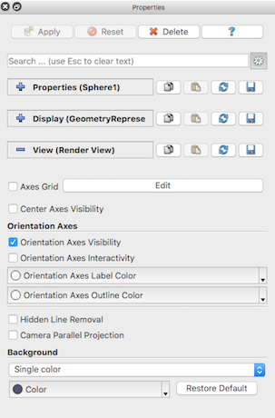
>>> view=GetActiveView()# Set center axis visibility>>> view.CenterAxesVisibility=0# Or you can use this variant to set the property on the active view.>>> SetViewProperties(CenterAxesVisibility=0)# Another way of doing the same>>> SetViewProperties(view,CenterAxesVisibility=0)# Similarly, you can change orientation axes related properties>>> view.OrientationAxesVisibility=0>>> view.OrientationAxesLabelColor=(1,1,1)
>>> displayProperties=GetDisplayProperties(source,view)# Both source and view are optional. If not specified, the active source# and active view will be used.# Now one can change properties on this object>>> displayProperties.Representation="Outline"# Or use the SetDisplayProperties API.>>> SetDisplayProperties(source,view,Representation=Outline)# Here too, source and view are optional and when not specified,# active source and active view will be used.
help 関数を使用すると、表示プロパティオブジェクトで使用可能なプロパティに関する情報をいつでも取得できます。
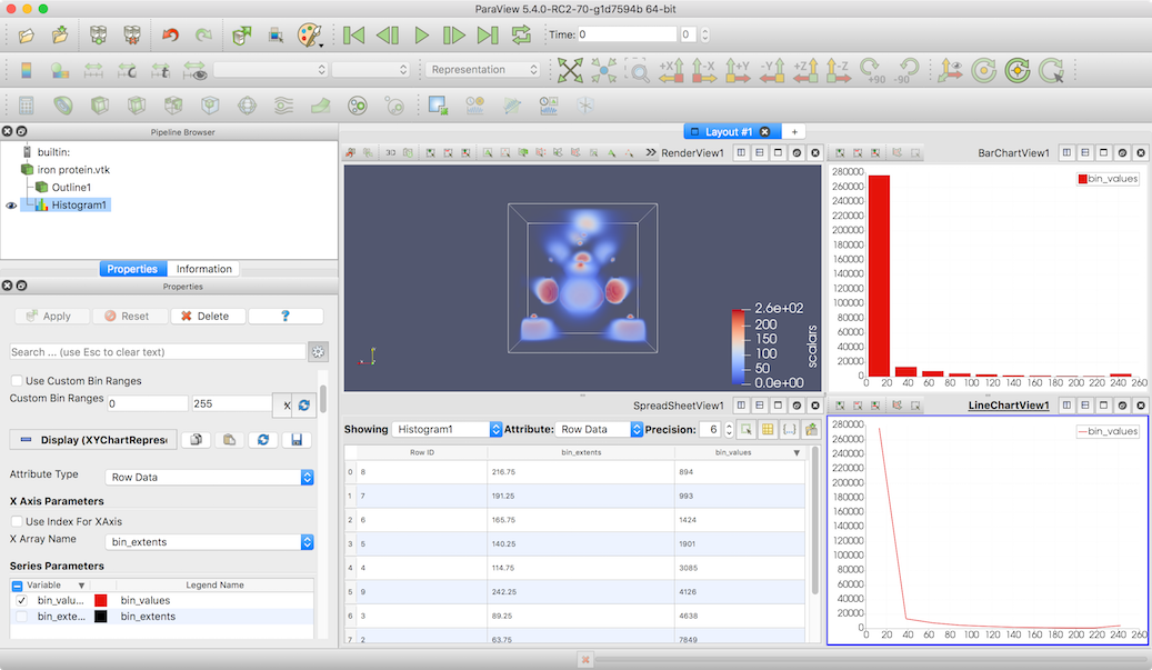
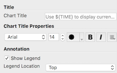
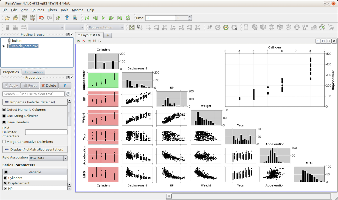
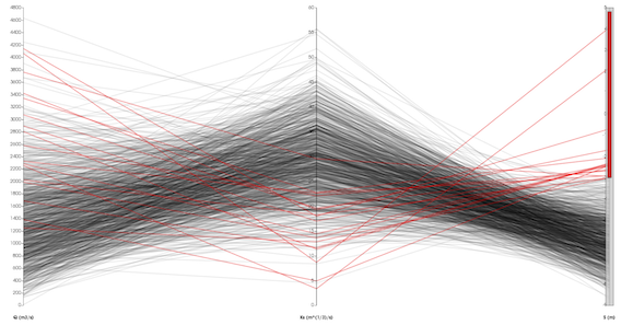
Display properties allow you to setup which series or data arrays are plotted in
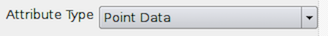
this view. You start by picking the AttributeType . Select the attribute
type that has the arrays of interest. For example, if you are plotting arrays
associated with points, then you should pick PointData .) Arrays with
different associations cannot be plotted together. You may need to apply filters
such as CellDatatoPointData or PointDatatoCellData to convert
arrays between different associations to do that.
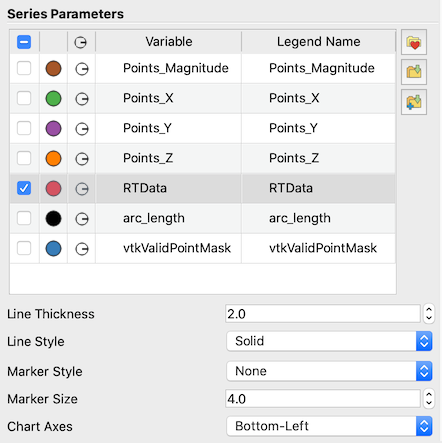
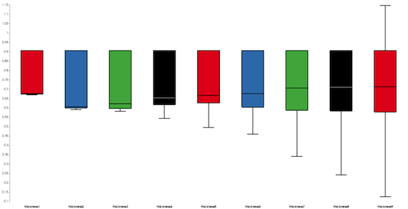
SeriesParameters control series or data arrays plotted on the Y-axis. All
available data arrays are lists in the table widget that allows you to
check/uncheck a series to plot in the first column. The second column in the
table shows the associated color used to plot that series. You can double-click
the color swatch to change the color to use. By default, ParaView will try to
pick a palette of discrete colors. The third column lets you set the
opacity of the series plot elements. The fourth column (Variable) shows the
name of the variable to plot. The fifth column (LegendName) shows the label to use for
that series in the legend. By default, it is set to be the same as the array
name. You can double-click to change the name to your choice, e.g., to add units.
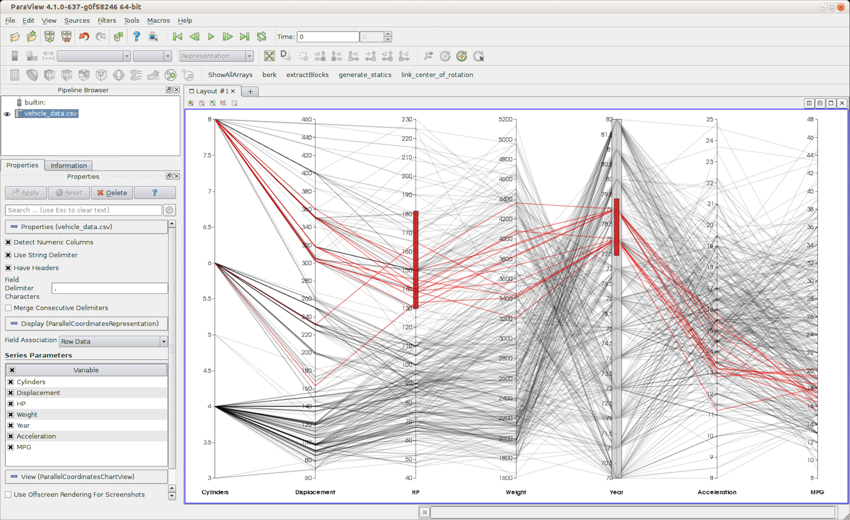
Other series parameters include LineThickness, LineStyle, MarkerStyle, and MarkerSize. To change any of these, highlight a row in The
SeriesParameters widget, and then change the associated parameter to affect
the highlighted series. You can change properties for multiple series and can select
multiple of them by using the CTRL (or ⌘) and ⇧ keys.
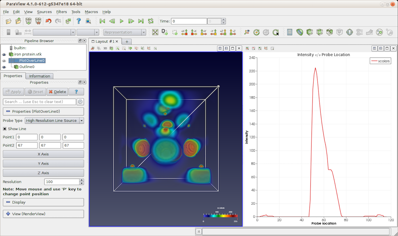
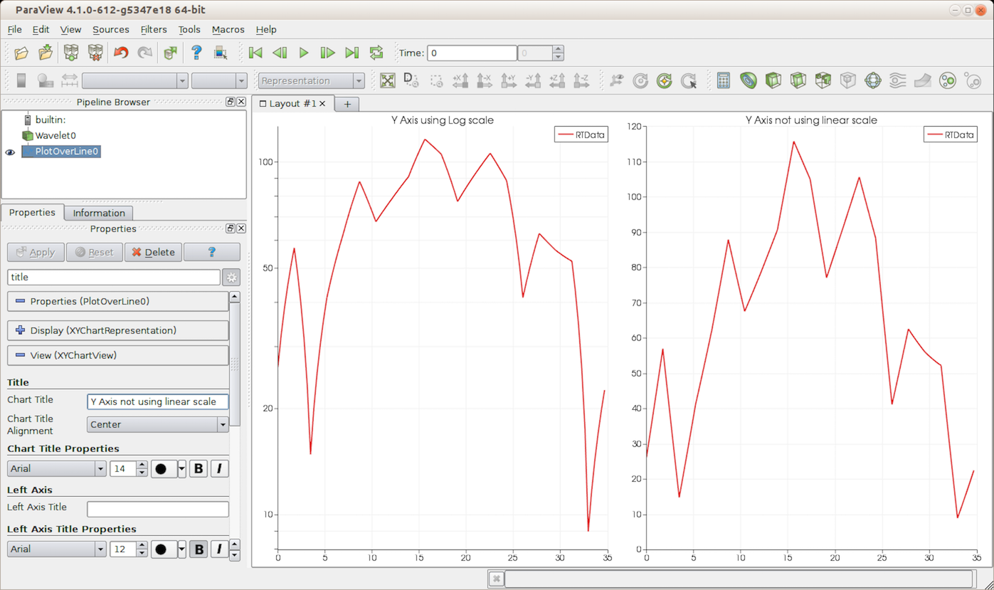
>>> fromparaview.simpleimport*# Create a data source to probe into.>>> Wavelet()<paraview.servermanager.Wavelet object at 0x1156fd810># We update the source so that when we create PlotOverLine filter# it has input data available to determine good defaults. Otherwise,# we will have to manually set up the defaults.>>> UpdatePipeline()# Now, create the PlotOverLine filter. It will be initialized using# defaults based on the input data.>>> PlotOverLine()<paraview.servermanager.PlotOverLine object at 0x1156fd490># Show the result.>>> Show()<paraview.servermanager.XYChartRepresentation object at 0x1160a6a10># This will automatically create a new Line Chart View if the# the active view is no a Line Chart View since PlotOverLine# filter indicates it as the preferred view. You can also explicitly# create it by using CreateView() function.# Display the result.>>> Render()# Access display properties object.>>> dp=GetDisplayProperties()>>> print(dp.SeriesVisibility)['arc_length', '0', 'RTData', '1']# This is list with key-value pairs where the first item is the name# of the series, then its visibility and so on.# To toggle visibility, change this list e.g.>>> dp.SeriesVisibility=['arc_length','1','RTData','1']# Same is true for other series parameters including series color,# line thickness etc.# For series color, the value consists of 3 values: red, green, and blue# color components.>>> print(dp.SeriesColor)['arc_length', '0', '0', '0', 'RTData', '0.89', '0.1', '0.11']# For series labels, value is the label to use.>>> print(dp.SeriesLabel)['arc_length', 'arc_length', 'RTData', 'RTData']# e.g. to change RTData's legend label, we can do something as follows:>>> dp.SeriesLabel[3]='RTData -- new label'# Access view properties object.>>> view=GetActiveView()# or>>> view=GetViewProperties()# To change titles>>> view.ChartTitle="My Title">>> view.BottomAxisTitle="X Axis">>> view.LeftAxisTitle="Y Axis"
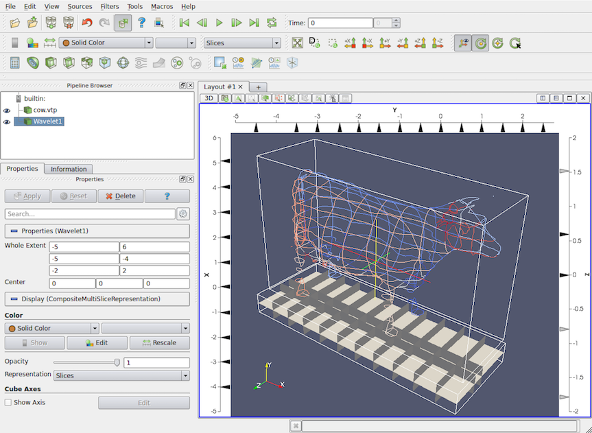
# To create a slice view in use:>>>view=CreateView("MultiSlice")# Use properties on view to set/get the slice offsets.>>>view.XSliceValues=[-10,0,10]>>>print(view.XSliceValues)[-10,0,10]# Similar to XSliceValues, you have YSliceValues and ZSliceValues.>>>view.YSliceValues=[0]>>>view.ZSliceValues=[]
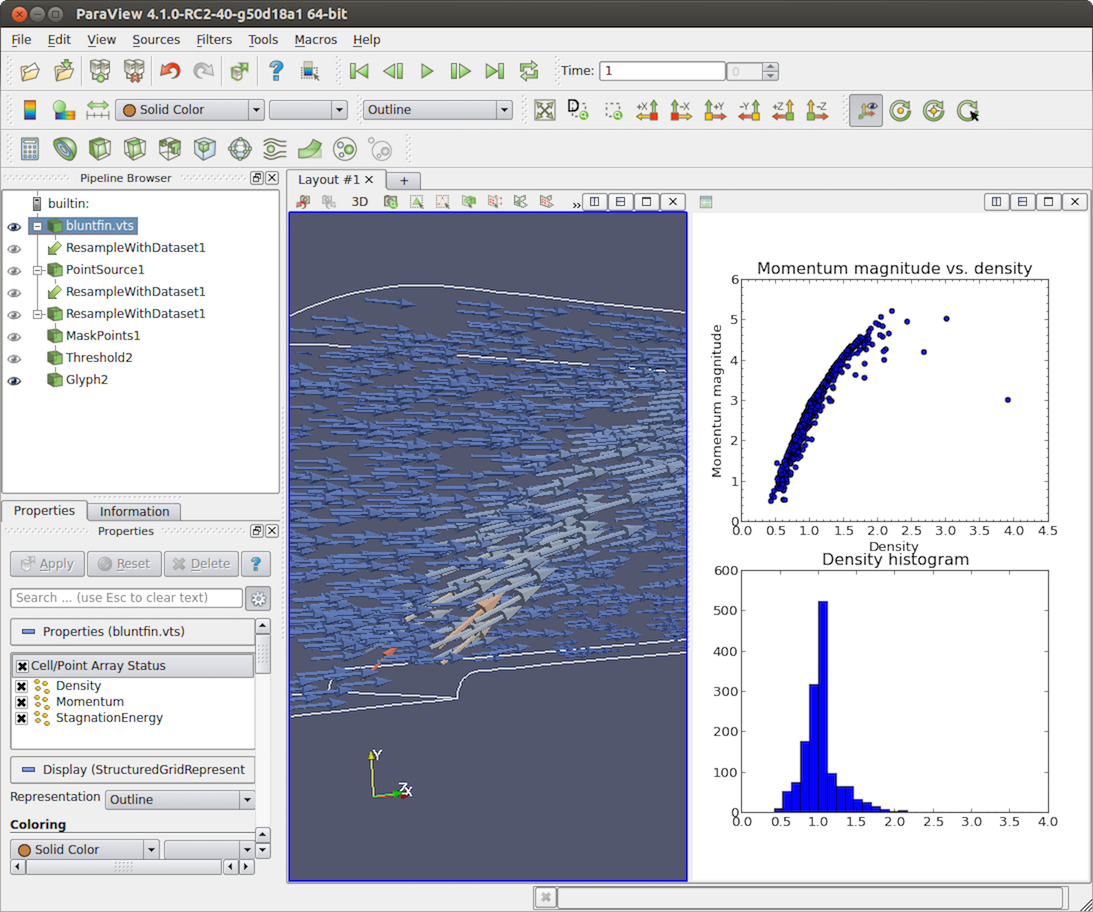
defsetup_data(view):# Iterate over visible data objectsforiinrange(view.GetNumberOfVisibleDataObjects()):# You need to use GetVisibleDataObjectForSetup(i)# in setup_data to access the data object.dataObject=view.GetVisibleDataObjectForSetup(i)# The data object has the same data type and structure# as the data object that sits on the server. You can# query the size of the data, for instance, or do anything# else you can do through the Python wrapping.print('Memory size: {0} kilobytes'.format(dataObject.GetActualMemorySize()))# Clean up from previous calls here. We want to unset# any of the arrays requested in previous calls to this function.view.DisableAllAttributeArrays()# By default, no arrays will be passed to the client.# You need to explicitly request the arrays you want.# Here, we'll request the Density point data arrayview.SetAttributeArrayStatus(i,vtkDataObject.POINT,"Density",1)view.SetAttributeArrayStatus(i,vtkDataObject.POINT,"Momentum",1)# Other attribute arrays can be set similarlyview.SetAttributeArrayStatus(i,vtkDataObject.FIELD,"fieldData",1)
GetVisibleDataObjectForSetup(visibleObjectIndex) -
This returns the visibleObjectIndex'th visible data object in
the view. (The data object will have an open eye next to it in the
PipelineBrowser .)
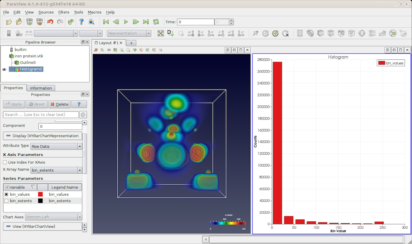
defrender(view,width,height):figure=python_view.matplotlib_figure(width,height)ax=figure.add_subplot(1,1,1)ax.minorticks_on()ax.set_title('Plot title')ax.set_xlabel('X label')ax.set_ylabel('Y label')# Process only the first visible object in the pipeline browserdataObject=view.GetVisibleDataObjectForRendering(0)x=dataObject.GetPointData().GetArray('X')# Convert VTK data array to numpy array for plottingfromparaview.numpy_supportimportvtk_to_numpynp_x=vtk_to_numpy(x)ax.hist(np_x,bins=10)returnpython_view.figure_to_image(figure)
This definition of the render(view,width,height) function
creates a histogram of a point data array named X from the first
visible object in the PipelineBrowser . Note the conversion
function, python_view.figure_to_image(figure) , in the last line.
This converts the matplotlib Figure object created
with python_view.matplotlib_figure(width,height) into a
vtkImageData object suitable for display in the viewport.
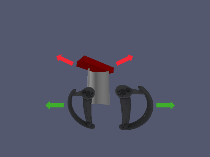
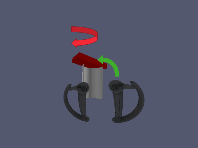
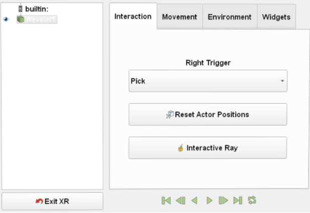
Trigger actions are assigned to the right trigger by default and include grabbing,
picking, probing, interactive clipping, teleportation, and adding points to sources
(such as a polyline source). The current action can be chosen via the XR menu
(see 4.14.3 章).
Adding points to a source --- 右のトリガーを押すと、右のコントローラーの先端に点が配置されます。ポリラインソースなど、アクティブソースが点の配置を許可している場合のみ有効です。
Pipeline Browser --- This is the same PipelineBrowser present in ParaView.
The visibility for each item in the pipeline can be modified by pointing the
navigation ray on the eye icon and pressing the right trigger.
Panels --- VR options are distributed into 4 panels, that can be displayed by
clicking on the corresponding tab:
Interaction --- This panel contains options related to the interactions with
the scene using the controllers (see 4.14.3.1 章).
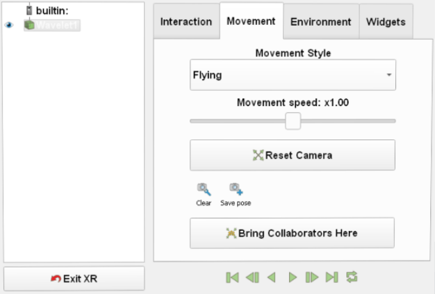
Movement --- This panel contains options related to the camera movement and
poses (see 4.14.3.2 章).
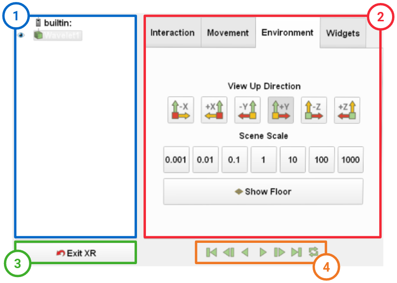
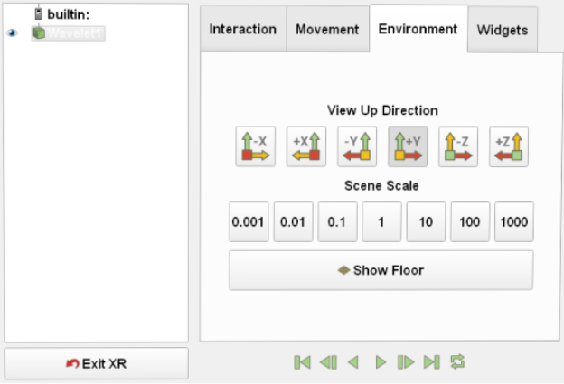
Environment --- This panel contains global options related to the scene
(see 4.14.3.3 章).
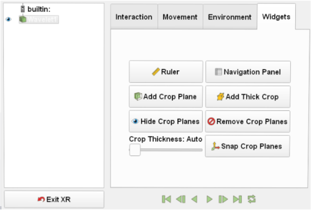
Widgets --- This panel contains options related to VR-specific widgets
(see 4.14.3.4 章).
Exit XR --- This button closes the current XR View.
Animation Buttons --- These buttons are used to navigate timesteps for
temporal datasets.
Clear --- This button clears all previously saved camera poses.
Savepose --- This button saves the current pose in the list of saved
camera poses. Up to 6 poses can be saved this way. For each saved pose, a
dedicated button is added to the right of this button.
図 4.32 Environment panel of the XR integrated menu.
ViewUpDirection --- These buttons set which axis points upwards from
the top of the HMD. This is useful when datasets or skyboxes are oriented
differently from the default.
SceneScale --- These buttons change the scaling factor of the scene.
A higher value results in all objects appearing larger.
ShowFloor --- This button allows hiding or showing the floor as a white plane.
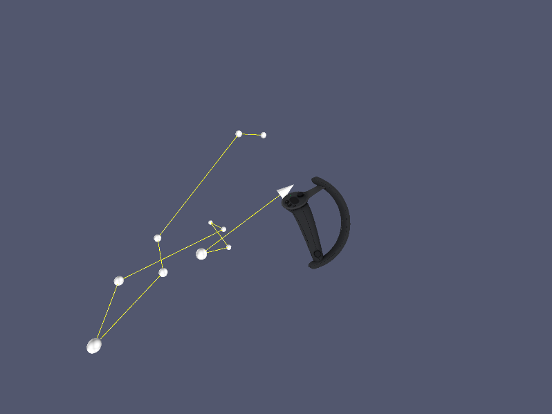
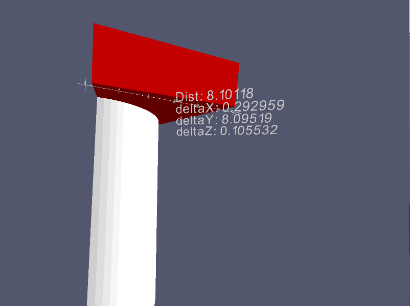
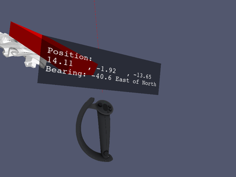
DistanceWidget --- This button adds a measuring tool to the scene.
Press the right trigger once to place the starting point where the right
controller is located, then press a second time with the controller at the
desired location to place the second point. Four values are displayed next
to the tool: distance and X, Y, Z difference between both points.
The tips of the line can be grabbed and moved individually after placing them.
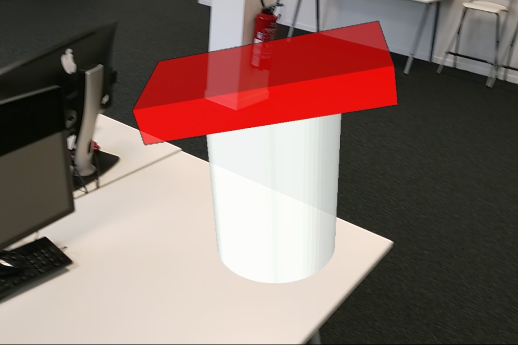
Cropping buttons --- The following buttons provide tools to crop data in real time.
Cropping planes can be moved by placing the right controller on them and grabbing
them with the right trigger. More than one plane can be added to the scene.
AddCropPlane --- シーンに切り出し平面を追加するボタンです。
AddThickCrop --- シーンに厚みを持つクロップ面を追加するボタンです。
HideCropPlanes --- This button hides all cropping planes in the scene.
CropThickness --- This horizontal slider sets the thickness of created
thick cropping planes (this parameter does not affect current ones). By default,
the value is set to auto, which adjusts the plane thickness according to the
current scene scale.
SnapCropPlanes --- This button allows to choose whether the cropping
planes should snap to the coordinates axes.
The remoting feature is only available on Windows for the Hololens 2 and requires an additional
package named Microsoft.Holographic.Remoting.OpenXr. With this, ParaView can connect to
another application in the remote device if both applications use the same version
of this package.
Note that the ParaView release uses the same version as the official player application developed
by Microsoft, available in the Microsoft Store, which is version 2.9.2.
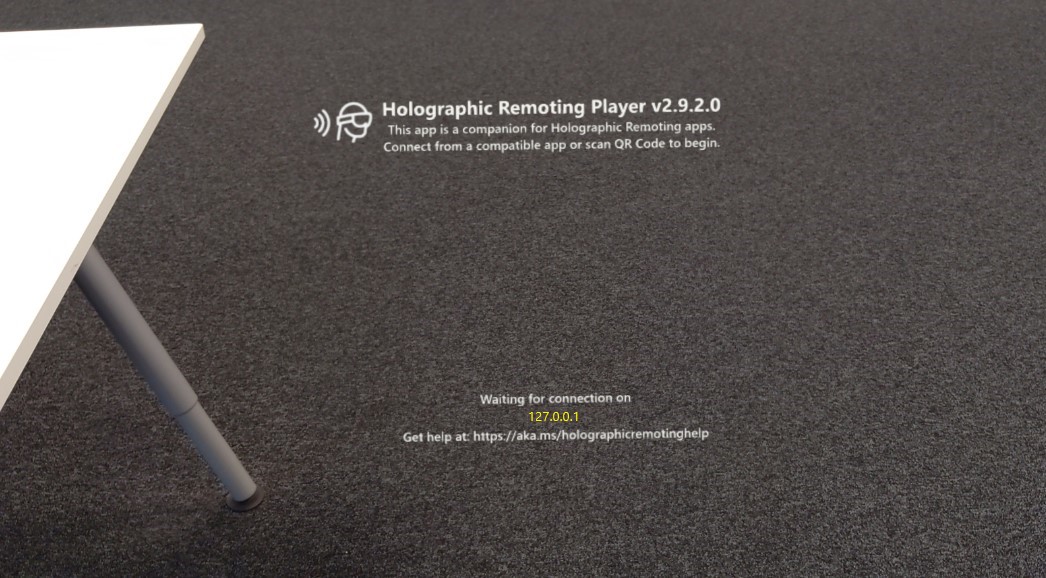
If you do have not an application already deployed in the remote device, we recommend downloading the
Holographic Remoting Player application in the Microsoft Store.
First, start the application on the remote device.
After launching this application, it will wait for another application to connect to it via an IP address.
図 4.36 Remote application awaiting connection in the Hololens 2.
You can now start ParaView and do any process on your data that you want. When you are ready to test it in
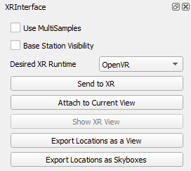
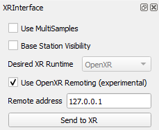
the Hololens 2, enable the XR Interface plugin. You will need to set different options:
DesiredXRRuntime --- set it to OpenXR because the Microsoft.Holographic.Remoting.OpenXr depends on it.
UseOpenXRRemoting --- enable or disable the remoting support.
Remoteaddress --- set the IP address to connect ParaView and the application in the Hololens 2.
図 4.37 XRInterface panel with OpenXR Remoting options.
After setting these options, you can click on SendToXR. Once the connection is established, you will be able
to see and interact with your dataset.
 ボタンを使用します。タブを閉じるには、
 ボタンをクリックし、そのタブにレイアウトされたすべてのビューを破棄します。タブ全体を別ウィンドウとしてポップアウトさせるには、タブバーの
  ボタンを使用します。
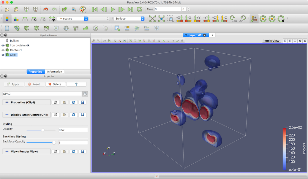
 ボタンを使ってパネルに高度なプロパティを表示するか、検索ボックスを使って名前で検索する必要があるかもしれません。
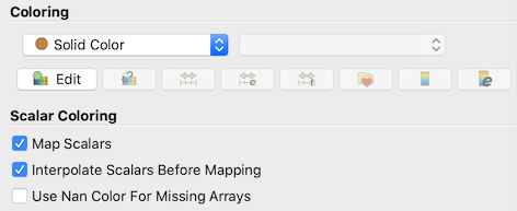

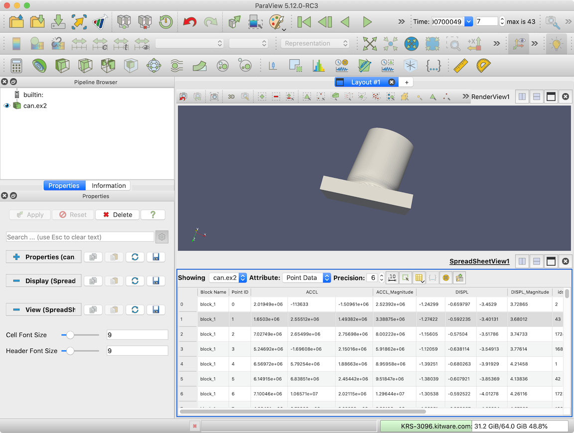
 ボタンを使用すると、表示する列を選択することができます。ボタンをクリックするとポップアップメニューが表示され、表示/非表示の列をチェック/アンチェックすることができます。
 ボタンをチェックすると、各セルを形成するポイントIDを見ることができるようになります。
 ボタンを使って、ビューに選択された要素のみを表示させます。他のビューで選択すると、この